Finite Element Analysis Post-Processing : User-Defined Scalar Fields
Import meshes and visualize arbitrary nodal scalar data without requiring external analysis software.
This tutorial demonstrates how to Generate contour plots directly from
- Mathematical functions
- Sensor measurements
- Experimental data
- Optimization results
- Scientific simulations
- Custom datasets
Normal Stress Distribution.
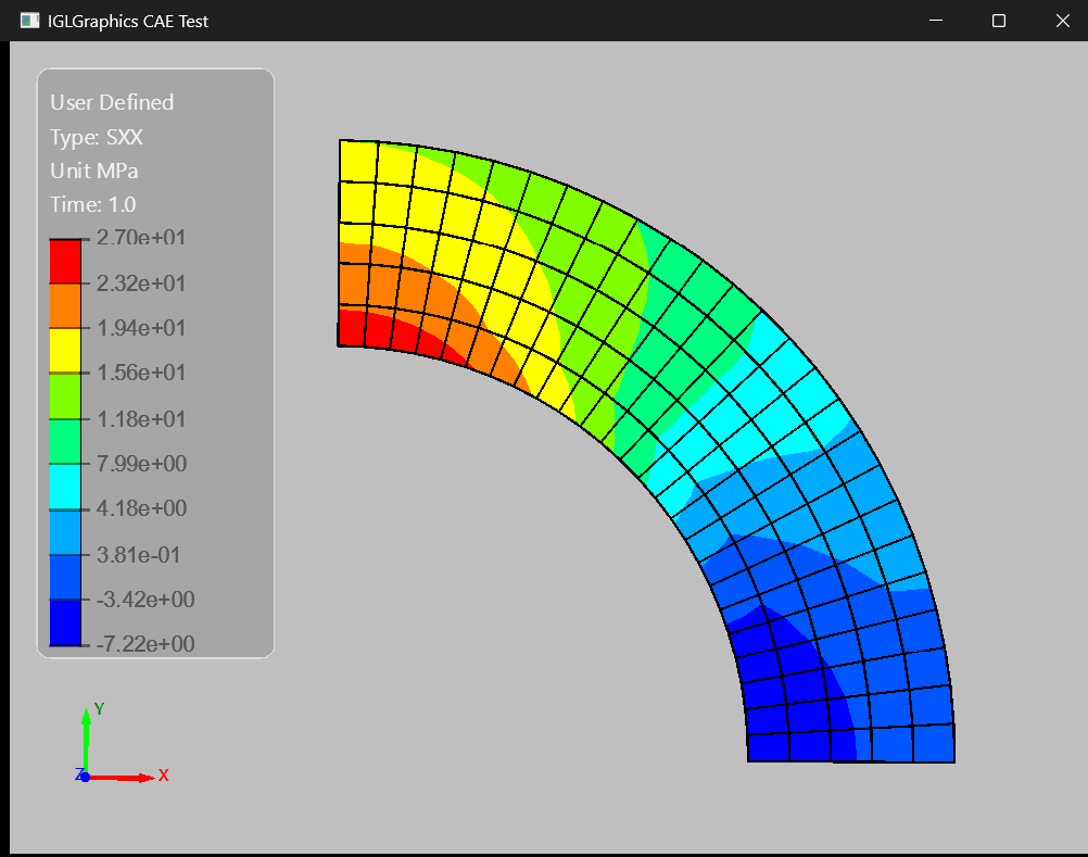
This example demonstrates how to visualize a user-defined nodal scalar field on a finite element mesh. The mesh is loaded independently, scalar values are read from an external file, and the contour legend is configured using custom result information. Finally, the scalar values are mapped onto the mesh and displayed as a contour plot using the IGLCAE post-processing framework.
# Step-1
#========================================================
wglcae = IGLCAE()
wglcae.SetContext(thecontext)  # Set the display context for the CAE model
wglcae.LoadModel(r"Pipe/2DPipe.msh")

# Step-2
#========================================================
file = r"Pipe/pipe_sxx.txt"
data = IGLFEAModel.ReadNodalArray(file)

title = 'User Defined'
resname = 'SXX'
units = 'MPa'
antime = 1.0

min_val = float(data.min())
max_val = float(data.max())

wglcae.SetScalaBarProps(title, resname, "", units, antime, min_val, max_val)
wglcae.DisplayContour(data)

# Set the central widget of the main window to the IGLViewer
win.setCentralWidget(view)
Mathematical Function
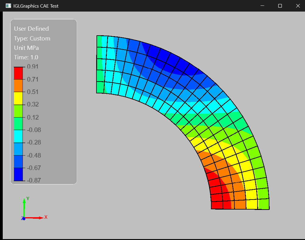
This example demonstrates how to generate and visualize a custom contour field directly from mesh geometry. The nodal coordinates are used to compute a mathematical scalar field using sine and cosine functions, creating a smooth spatial variation across the model. The computed values are then displayed as contours on the mesh with a user-defined legend, independent of any FEA result file.
# Step-1
#========================================================
wglcae = IGLCAE()
wglcae.SetContext(thecontext)  # Set the display context for the CAE model
wglcae.LoadModel(r"Pipe/2DPipe.msh")

# Step-2
#========================================================
mesh = wglcae.GetMeshDS()
nodes = mesh.GetNodes()

x = nodes[:, 0]
y = nodes[:, 1]

data = (
    np.sin(x * 0.05) *
    np.cos(y * 0.05)
)

title = 'User Defined'
resname = 'Custom'
units = 'MPa'
antime = 1.0

min_val = float(data.min())
max_val = float(data.max())

wglcae.SetScalaBarProps(title, resname, "", units, antime, min_val, max_val)
wglcae.DisplayContour(data)

# Set the central widget of the main window to the IGLViewer
win.setCentralWidget(view)
Gaussian Distribution
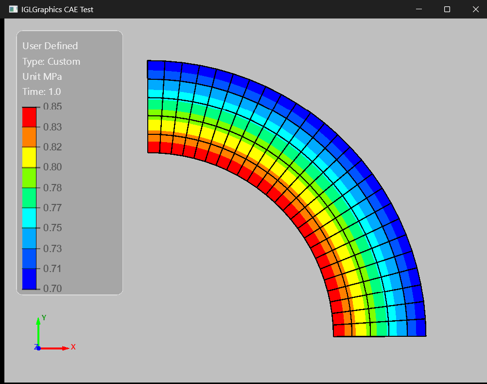
This example demonstrates how to create a Gaussian-style scalar field using the nodal coordinates of the mesh. The exponential function produces a smooth peak at the center that gradually decreases toward the boundaries, making it useful for testing contour visualization and color mapping. The generated values are then displayed as a contour plot with a custom legend and scalar range.
# Step-1
#========================================================
wglcae = IGLCAE()
wglcae.SetContext(thecontext)  # Set the display context for the CAE model
wglcae.LoadModel(r"Pipe/2DPipe.msh")

# Step-2
#========================================================
mesh = wglcae.GetMeshDS()
nodes = mesh.GetNodes()

x = nodes[:, 0]
y = nodes[:, 1]

data = np.exp(
    -(x*x + y*y)/10000
)

title = 'User Defined'
resname = 'Custom'
units = 'MPa'
antime = 1.0

min_val = float(data.min())
max_val = float(data.max())

wglcae.SetScalaBarProps(title, resname, "", units, antime, min_val, max_val)
wglcae.DisplayContour(data)

# Set the central widget of the main window to the IGLViewer
win.setCentralWidget(view)